December 2021 LIP of the Month
Investigating relationships between intraplate magmatism, upper-mantle temperature and lithospheric thickness.
P.W. Ball
Extracted and revised from: Ball, P. W., White, N. J., Maclennan, J., & Stevenson, S. N. (2021). Global influence of mantle temperature and plate thickness on intraplate volcanism. Nature Communications, 12(2045), 1–13.
Introduction
The thermochemical structure of lithospheric and asthenospheric mantle exert primary controls on surface topography and volcanic activity. Volcanic rock compositions and mantle seismic velocities provide indirect observations of this structure. In this study, a global database that consists of >20, 000 geochemical analyses of Neogene-Quaternary intraplate volcanic rocks was compiled ( <10 Ma and located <400 km from where they were erupted). In the next three sections, the spatial distribution and chemical compositions of these samples are compared to observations from upper-mantle tomographic models before both geochemical and tomographic databases are used to estimate mantle temperatures and lithospheric thicknesses beneath each volcanic province.
Spatial Distribution of Present-Day Intraplate Magmatism
Intraplate volcanism is concentrated within regions where negative shear-wave velocity anomalies occur at depths of 150 ± 25 km in the SL2013sv tomographic model (Figure 1a; Schaeffer and Lebedev, 2013). Slow velocities at 150 ± 25 km depth correspond to regions of thin lithosphere if SL2013sv is converted into an estimate of mantle temperature (Figure 1b; Hoggard et al., 2020). These visual associations can be quantified formally. 89% of Earth’s surface that is covered by intraplate volcanism occurs in regions underlain by negative values of ΔVs whose areal distribution only constitutes 61% of global area (Figure 2a). Ninety-five percent of Earth’s surface that is covered by intraplate volcanism occurs in regions underlain by continental lithosphere <100 km thick whose areal distribution constitutes 62% of global area (Figure 2b). Using a Kolmogorov–Smirnov test, the probability that co-location of intraplate samples, negative values of ΔVs, and anomalously thin continental lithosphere arises from chance is <1 in 10100.
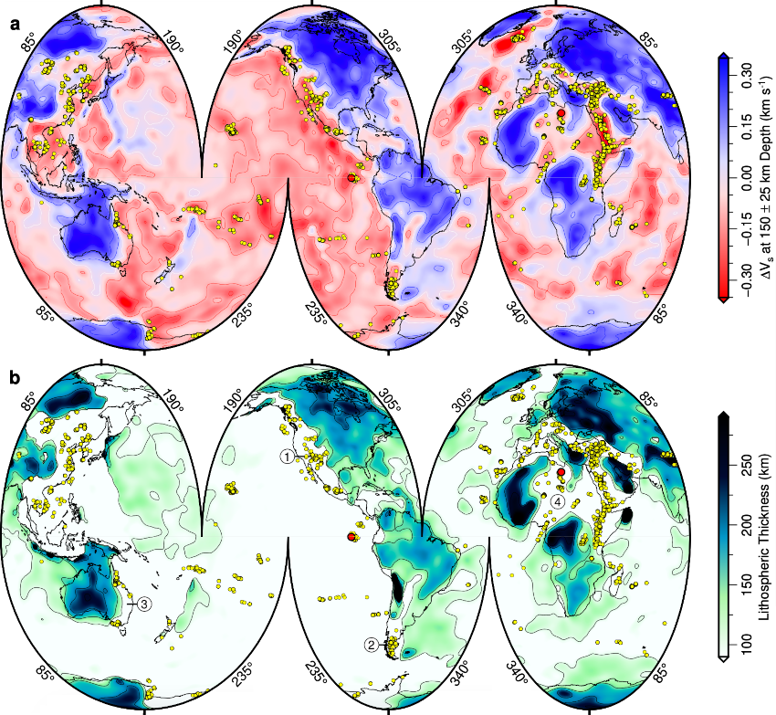
Figure 1 – a) Segmented Mollweide projection of globe showing average value of shear-wave velocity anomaly, ΔVs, taken from SL2013sv tomographic model at depth of 150 ± 25 km. Red/white/blue contours = positive/zero/negative values of ΔVs plotted at intervals of 0.1 km s−1; yellow circles = loci of intraplate magmatic samples in filtered database. b) Spatial variation of lithospheric thickness calculated using intersection of 1175 °C isothermal surface from SL2013sv tomographic model that is converted into temperature. Black contours = thickness values at intervals of 50 km.
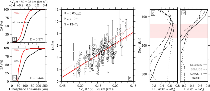
Figure 2 – a) Percentage cumulative area, ΣA, plotted as function of average value of ΔVs from SL2013sv tomographic model at depths of 150 ± 25 km where globe is subdivided into 1° bins weighted according to cos?? where ? = latitude in degrees; black curve = cumulative areal distribution of ΔVs; red line = cumulative areal distribution of binned intraplate volcanic samples; black/red numbered dashed lines = percentages of global surface and of intraplate volcanism with ΔVs < 0 km s−1; D = value of Kolmogorov–Smirnov statistic. b) ΣA plotted as function of lithospheric thickness. Black/red lines = cumulative areal distribution of lithospheric thickness and of binned intraplate volcanic samples, respectively; black/red numbered dashed lines = percentages of global surface and of intraplate volcanism with lithosphere <100 km thick. c) La/Sm plotted as function of average value of ΔVs at depths of 150 ± 25 km from SL2013sv tomographic model. Circles and error bars = average value ± σ for each 1° bin; red line = line that best fits values weighted according to cos??; pair of dotted red lines = uncertainty envelope for suite of best-fit lines where filtered database is binned using 99 different configurations spaced at 0.1° intervals; R = correlation coefficient and its uncertainty; P = population correlation coefficient; N = number and range of bins. d) Value of R, calculated between La/Sm and ΔVs, plotted as function of depth for four different tomographic models. Solid/dash-dot/dashed/dotted lines = SL2013sv/CAM2016Vsv/SEMUCB-WM1/S40RTS tomographic models; R = 0.28 is minimum value of R distinguishable from zero at significance level of =0.001. Red dashed line with shaded rectangle = 150 ± 25 km for reference. e) Value of R, calculated between lithospheric thickness and ΔVs, plotted as function of depth as before.
Relationships Between Igneous Rock Geochemistry and Upper-Mantle Tomography
The relationship between La/Sm and ΔVs is a useful way to explore the role that sub-plate thermal anomalies play in generating intraplate volcanism. To ensure observed La/Sm ratios are close to those of primitive melts, all samples that have MgO contents <9 wt% and >14.5 wt% are excised from the database. For ease of analysis and to mitigate the influence of local compositional heterogeneity, Earth’s surface is subdivided into 1° × 1° bins and only bins with >5 samples that have been analyzed for La and Sm concentrations are exploited. Average La/Sm and ΔVs measurements for each bin are compared and the Pearson product-moment correlation coefficient, R, between these measurements is calculated (Figure 2c).
There is a positive correlation between La/Sm ratios and ΔVs values for the SL2013sv tomographic model at a depth of 150 ± 25 km (R = 0.65 ± 0.07; Fig. 2c). Thus, igneous rocks with lower La/Sm ratios, which are indicative of higher melt fractions, coincide with regions with lower values of ΔVs at a depth of 150 ± 25 km, which are indicative of higher temperatures at this depth. In Fig. 2d, correlations between La/Sm and ΔVs are shown as a function of depth for the SL2013sv, CAM2016Vsv, SEMUCB-WM1 and S40RTS global tomographic models (Ritsema et al., 2011; Schaeffer and Lebedev, 2013; French & Romanowicz, 2014; Ho et al., 2016). In each case, the value of R is greatest between 100 and 200 km depth. For three of these models, the value of R sharply decreases at depths of >250 km. Since both La/Sm and ΔVs are expected to decrease as mantle temperature increases, these observations suggest that intraplate volcanic compositions are sensitive to temperature variations within the uppermost mantle.
Estimating Mantle Temperatures and Lithospheric Thicknesses
Spatial and chemical correlations between intraplate magmatism and seismic tomography can be investigated further by comparing estimates of asthenospheric potential temperature, Tp, generated using each dataset. First, the chemical composition of intraplate volcanic rocks is used to constrain the depth and degree of mantle melting. A geochemical inverse modeling strategy is exploited which minimizes the misfit between observed concentrations of rare earth elements and those generated using a peridotite melting paramterization at a range of Tps and lithospheric thicknesses (INVMEL; McKenzie and O’Nions, 1991). These values can be directly compared with asthenospheric temperatures and with plate thicknesses obtained from tomographic models that have been converted into temperature. Here, geochemical estimates of Tp are compared with values determined at 150 ± 25 km depths for the SL2013sv model (Hoggard et al., 2020). Both geochemical and tomographic schemes are applied to each 1°x1° bin in the filtered database. Globally, a positive correlation coefficient of R = 0.54 is observed between geochemical and tomographic estimates of ΔTp, which is the temperature anomaly with respect to ambient asthenospheric mantle for each modeling technique (Figure 3).
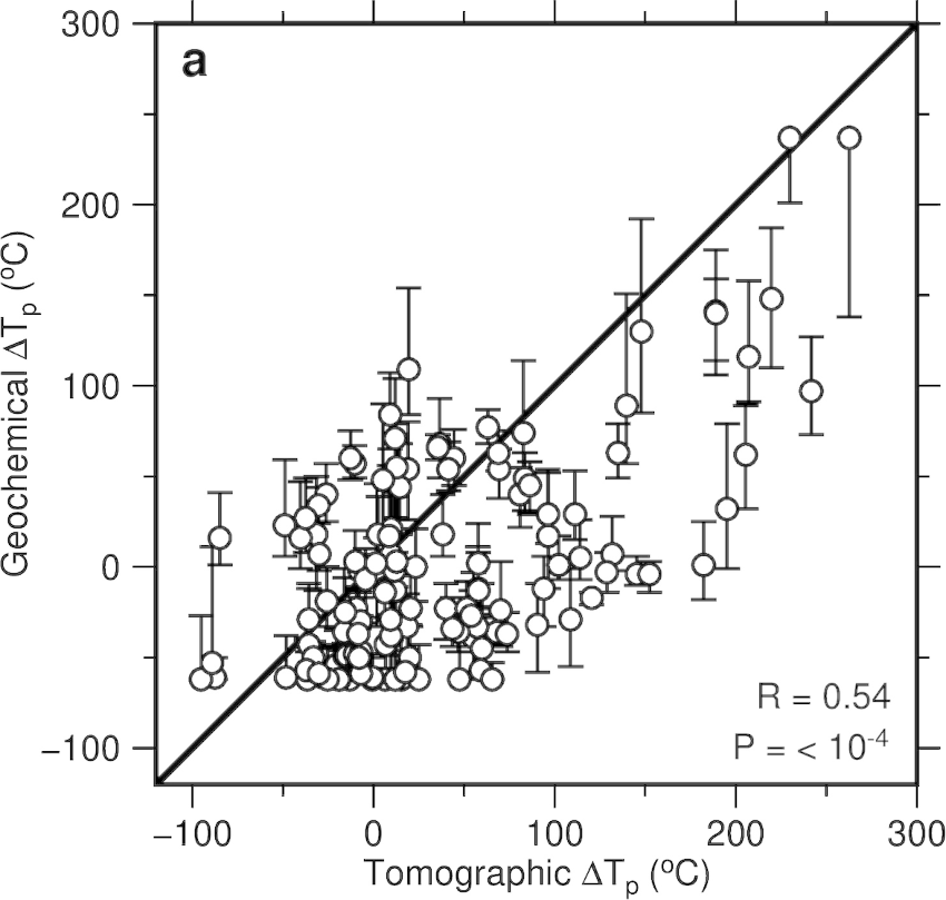
Figure 3 - Diagram showing relationship between ΔTp determined by geochemical inverse modeling and that determined by calibration of SL2013sv tomographic model where ambient mantle temperatures are assumed to be 1312 °C and 1333 °C, respectively. Open circles with vertical and horizontal error bars = calculated values of temperature for global distribution of intraplate volcanism ± 1.5× minimum misfit; black line 1:1 relationship; R = correlation coefficient; P = population correlation coefficient.
Implications for Mantle Temperatures Through Time
Intraplate magmatism, positive asthenospheric temperature anomalies and thinned lithosphere are closely related during Neogene-Quaternary times. Asthenospheric temperature variation and lithospheric thickness changes can generate vertical motions of the order of hundreds of meters at the Earth’s surface that are superimposed on motions generated by mantle convection. Since intraplate magmatism occurs throughout the stratigraphic record, a combined analysis of igneous rocks and stratigraphy could help to elucidate the history of mantle convective and dynamic topographic phenomena throughout the Phanerozoic Era.
References
McKenzie, D. & O’Nions, R. K. Partial melt distributions from inversion of rare-earth element concentrations. J. Petrol. 32, 1021–1091 (1991).
Ritsema, J., Deuss, A., Van Heijst, H. & Woodhouse, J. S40RTS: a degree-40 shear-velocity model for the mantle from new Rayleigh wave dispersion, teleseismic traveltime and normal-mode splitting function measurements. Geophys. J. Int. 184, 1223–1236 (2011).
French, S. W. & Romanowicz, B. A. Whole-mantle radially anisotropic shear velocity structure from spectral-element waveform tomography. Geophys. J. Int. 199, 1303–1327 (2014).
Ho, T., Priestley, K. & Debayle, E. A global horizontal shear velocity model of the upper mantle from multimode Love wave measurements. Geophys. J. Int. 207, 542–561 (2016).
Hoggard, M. J. et al. Global distribution of sediment-hosted metals controlled by craton edge stability. Nat. Geoscience 13, 504–510 (2020).